Python profiling.sampling: technical guide to Tachyon, GIL, flame graphs and production profiles

Python 3.15 adds a meaningful new surface for performance engineering: profiling.sampling, a Tachyon-based statistical profiler that can attach to live Python processes, sample them with different clocks and expose both interactive and replayable views. It is not merely “another profiler.” It changes how standard Python tooling can participate in production debugging, postmortem analysis and shared performance workflows.

This article assumes familiarity with CPU profiling, call stacks, the GIL, concurrency and production services. The goal is not to repeat command help. It is to place profiling.sampling on the technical map: what model it uses, which decisions its flags imply, when to prefer it over tracing, which biases sampling still carries and how to integrate it without turning every performance incident into an unrepeatable one-off capture.

From profiling as a package to Tachyon as the backend

PEP 799 formalized a transition that had been building for years. Rather than leaving profiling tools scattered under historical names, Python now introduces a dedicated profiling package, adds profiling.tracing as the modern replacement for legacy deterministic profilers and uses profiling.sampling for low-intrusion statistical work. The profile documentation already reflects that split: profile is deprecated in 3.15, profiling.tracing is recommended for development and tests, and profiling.sampling for production debugging.

The sampling backend is Tachyon. The documented interface is intentionally CLI-oriented and artifact-oriented: attach, observe, record and replay. That tells us something about the expected use case. This is process inspection tooling, not merely a helper around a function call in a benchmark harness.

The documentation also states that the profiled process runs “without overhead” because it does not require instrumentation. The accurate reading is narrower than the slogan. The sampler itself still consumes resources as an external process and observation is never physically free. What disappears is in-process event-hook overhead, the very cost that makes deterministic tracers harder to use against live production workloads without changing the thing being measured.

Capture model: attach, permissions and operational boundaries

The profiler attaches to an existing process by PID. The canonical example is:

python -m profiling.sampling live <pid>

The user needs the right permissions; attaching to another user’s process may require administrative privilege. That is not a footnote for production. Mature usage should define who is allowed to attach, on which hosts, how artifacts are retained and how the action is audited. A profiler that can inspect stack data is operationally powerful and should be governed like other diagnostic capabilities.

The command families are well chosen: live for interactive exploration, top for terminal summaries, record for persisted captures and replay for later review. In real incidents, record plus replay is usually the most defensible workflow. It preserves evidence, supports comparison, allows collaboration and survives after the spike or worker process is gone.

Clocks: cpu and wall answer different questions

The --clock option carries more semantic weight than many users expect. cpu samples actual CPU execution. wall samples elapsed real time, which means waiting, blocking and time off-CPU remain visible. Choosing the wrong clock can produce a technically correct answer to the wrong operational question.

If an API is slow because compression saturates cores, a CPU profile is likely to show the hotspot directly. If it is slow because threads wait on a database, a queue, a mutex or an external dependency, wall time is closer to the latency users experience. For mixed systems, capturing both is often more useful than arguing about which one is “the real profile.”

The --subprocesses option, documented for wall, matters for modern Python deployments. Workers, pools, helper binaries and hybrid architectures often push work into child processes. A profile that ignores children may describe only the most visible part of the cost rather than the total cost perceived by the request path.

Sampling frequency: resolution, cost and stability

profiling.sampling exposes --frequency, with a documented default of 100 Hz and an allowed range from 1 to 1000 Hz. More samples are not automatically better analysis.

At 100 Hz, a 30-second capture yields roughly 3000 observations, usually enough to expose stable hot paths in services with persistent behavior. Raising the frequency may help with shorter events or finer temporal resolution, but it increases data volume and system perturbation. Lowering it may be enough for long-running workloads where only a coarse distribution is needed. The right choice depends on the lifetime of the phenomenon under study, not on a reflex that says “higher must be safer.”

Sampling bias still exists. Very short work, bursts aligned with the sampling period or workload changes during the window can be missed or overrepresented. A beautiful flame graph does not rescue a poor capture. Repetition, multiple windows and correlation with service metrics remain part of good engineering practice.

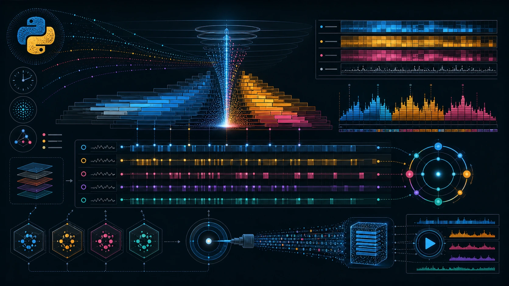
Views: when to use flamegraph, heatmap, gil, functions and stack

Each view is useful when it matches the question.

flamegraph

This is the strongest first view for hierarchy and concentration. Width represents sample frequency; height represents stack depth. It is excellent for spotting unexpected wide paths, serialization layers, parsers, framework wrappers or business loops that dominate a request. It is also the most communicable view when another team needs to understand where the time enters the system.

heatmap

The heatmap is best when behavior changes over time: warm-up, garbage collection, batch phases, startup effects, periodic degradation or load bursts. Aggregates can flatten those transitions; a heatmap exposes them.

gil

The GIL view helps surface functions that hold the interpreter lock for a meaningful share of the capture. In multi-threaded code, it separates “we have threads” from “we obtain useful parallel progress.” It does not replace architecture analysis, but it shortens the search when interpreter contention is part of the problem.

functions

The flat table is excellent for sorting, comparing and communicating priorities: user, library or system functions; self time versus aggregate contribution; direct cost versus caller-driven cost. It carries less causal context than a flame graph, but it is fast and operationally convenient.

stack

The stack view is appropriate when an immediate thread-by-thread snapshot matters more than aggregate statistics: live waiting, blocking inspection or a quick operational read.

The GIL: what the tool can show and what it cannot decide

The module makes a recurring Python question more approachable: “Are we limited by the GIL?” The gil view can reveal functions that hold the lock for a high share of the profile. That is useful when CPU-bound work runs inside threads, native extensions fail to release the lock or portions of code serialize progress unexpectedly.

But the conclusion is not automatic. A high GIL share alone does not prove the system should move to processes, asyncio or native extensions. First correlate it with throughput, latency, CPU utilization, queue depth and the actual service objective. In some I/O-bound workloads the signal may be unimportant. In others, one CPU-heavy hotspot explains nearly all scaling failure.

profiling.sampling is strongest when combined with metrics and, when needed, targeted instrumentation such as sys.monitoring or controlled tracing. Sampling tells you where to look. Directed instrumentation helps prove a narrower hypothesis.

How it compares with profiling.tracing, timeit and observability

Python 3.15 makes the tool split clearer:

• profiling.sampling: live-process inspection, low intrusion, production suitability, time distribution and hot paths.
• profiling.tracing: deterministic call-level detail, strong for development, tests and controlled analysis.
• timeit: repeatable micro-comparisons, not whole-system diagnosis.
• Metrics, logs and distributed traces: service behavior, component correlation and request-level context.

The classic mistake is trying to make one tool answer every question. A better workflow chains them. A latency alert leads to metrics. Metrics show CPU rising in one worker pool. A sampling profile identifies a hot path. A controlled trace or timeit experiment validates the refactor. Deployment is then confirmed by metrics again.

Profile files, reproducibility and data governance

record writes a binary profile and replay opens it later. That sounds like convenience, but in larger organizations it changes analysis quality. A recorded profile can be attached to a ticket, compared across releases, reviewed by another engineer and preserved as evidence of a regression.

Profiles can still expose module names, paths, symbols, function structure and architectural clues. They should not be treated as harmless logs. If stored outside the original environment, they belong under access, classification and retention policies. In regulated environments, an artifact may contain no personal data and still reveal sensitive implementation detail.

Sensible production integration

A mature integration does not mean leaving sampling on all the time. It means defining triggers and procedures.

• Capture during sustained latency incidents or reproducible regressions.
• Use short, declared windows with a frequency appropriate to the phenomenon.
• Record Python version, application release, host, clock, frequency, duration and approximate load.
• Store the profile beside contextual metrics so it is not interpreted without a baseline.
• Repeat the capture after the fix to demonstrate effect rather than rely on intuition.

In Kubernetes or ephemeral platforms, teams also need to decide where the tool lives: a privileged diagnostic container, a controlled node session or a temporary sidecar model, depending on policy. The Python documentation defines profiler semantics. Operational architecture remains the team’s responsibility.

Interpretation traps

Five common mistakes recur:

1. Mistaking width for guilt. A wide function may represent necessary work, not inefficient work.
2. Ignoring workload realism. A profile taken under unrealistic traffic describes another system.
3. Comparing incompatible captures. Changing clock, frequency or window and then comparing percentages as if nothing changed is fragile analysis.
4. Optimizing self time without looking at callers. Sometimes the issue is how often a function is invoked, not how it is implemented locally.
5. Treating one capture as a verdict. In performance work, repetition and context matter more than one dramatic image.

Facts, interpretation and projections

Verified facts

• Python 3.15.0b1 documentation describes profiling.sampling as a Tachyon-based statistical profiler.
• The tool supports live, top, record and replay; cpu and wall; and the views flamegraph, heatmap, gil, functions and stack.
• PEP 799 created the profiling package and reorganized the modern profiler stack under it.
• profile is deprecated in 3.15 and cProfile remains a backward-compatible alias of profiling.tracing.

Technical interpretation

• The main shift is not merely the presence of a sampler, but an officially documented path for inspecting production processes without relying exclusively on external tools.
• The record and replay workflow encourages reproducibility and collaborative review, two historically weak points in ad hoc performance investigations.

Reasonable projections

• If the API and formats stabilize well during the 3.15 cycle, internal tools, SRE playbooks and incident docs are likely to standardize around replayable profiles.
• The new package may also become a clearer educational entry point for separating benchmarking, tracing and sampling inside Python.

Conclusion

profiling.sampling fills a real gap between high-level observability and detailed tracing. For performance engineering, its value lies in reduced friction: attach, sample, persist, replay and discuss the same artifact. It does not remove statistical bias or replace judgment, but it reduces dependence on intuition, irreproducible captures and heterogeneous tooling.

The practical recommendation is straightforward. Use it for live-process distribution questions and hot paths. Keep profiling.tracing for controlled detail. Use timeit for micro-decisions. And preserve operational context around every capture. A good profiler does not replace a good method; it makes that method more effective.

FAQ

Does profiling.sampling replace cProfile?

Not entirely. cProfile remains available as a backward-compatible alias of profiling.tracing. Sampling and tracing answer different questions.

Which clock should I use first?

Start with cpu when you suspect CPU consumption. Capture wall too when investigating user-visible latency, waiting or blocking.

Is 100 Hz always enough?

Not always, but it is a sensible starting point. Adjust based on event duration, acceptable cost and the resolution you need.

Can I attach it to any process?

Only when the operating system allows access. Python documents that inspecting processes owned by another user may require administrative privilege.

Does the gil view prove I should abandon threads?

No. It shows GIL-holding concentration. Architectural decisions still require throughput, latency and workload analysis.

Sources

• Python 3.15: profiling.sampling.
• PEP 799: A dedicated profiling package.
• Python 3.15: profile and migration to profiling.tracing.
• Python 3.15: sys.monitoring.
• Python 3.15: timeit.
• Brendan Gregg: Flame Graphs.